JAX gradients#

Every public function in classy_szlite is JAX-traceable. :class:~classy_szlite.CosmoParams and :class:~classy_szlite.ProfileParamsA10 are JAX pytrees (NamedTuples of arrays), so you can differentiate w.r.t. any field directly.

Why this matters#

A pure-JAX forward model unlocks the entire JAX ecosystem on top of classy_szlite:

Fisher matrices — jax.jacfwd / jax.jacrev give exact per-parameter derivatives, so the Fisher information \(F_{ij}=\sum_\ell \partial_i C_\ell \,\mathrm{Cov}^{-1}_{\ell\ell'}\partial_j C_{\ell'}\) is one line.
Gradient-based sampling — Hamiltonian Monte Carlo / NUTS (numpyro, blackjax) need \(\nabla \log p\). We give it exactly, not via finite differences.
MAP — scipy.optimize.minimize (L-BFGS-B, etc.) with exact jax.grad gradients converges in ~20–40 forward+gradient evaluations (see Examples).

Finite differences are slow, noisy, and require choosing \(\varepsilon\). Autodiff is exact (up to floating point) and costs roughly the same as the forward pass.

Verification: autodiff vs finite difference#

The plot below shows two things at once:

Left — \(D_\ell^{yy}(P_0)\) at \(\ell = 1500\) as \(P_0\) varies, with tangent lines whose slopes were computed by jax.grad. They sit exactly on the curve, which means autodiff is consistent with the forward pass.
Right — gradient values from jax.grad (solid line) compared to a 2-point central finite difference with \(\varepsilon = 10^{-3}\) (open circles). The two agree to numerical precision.

autodiff vs finite difference

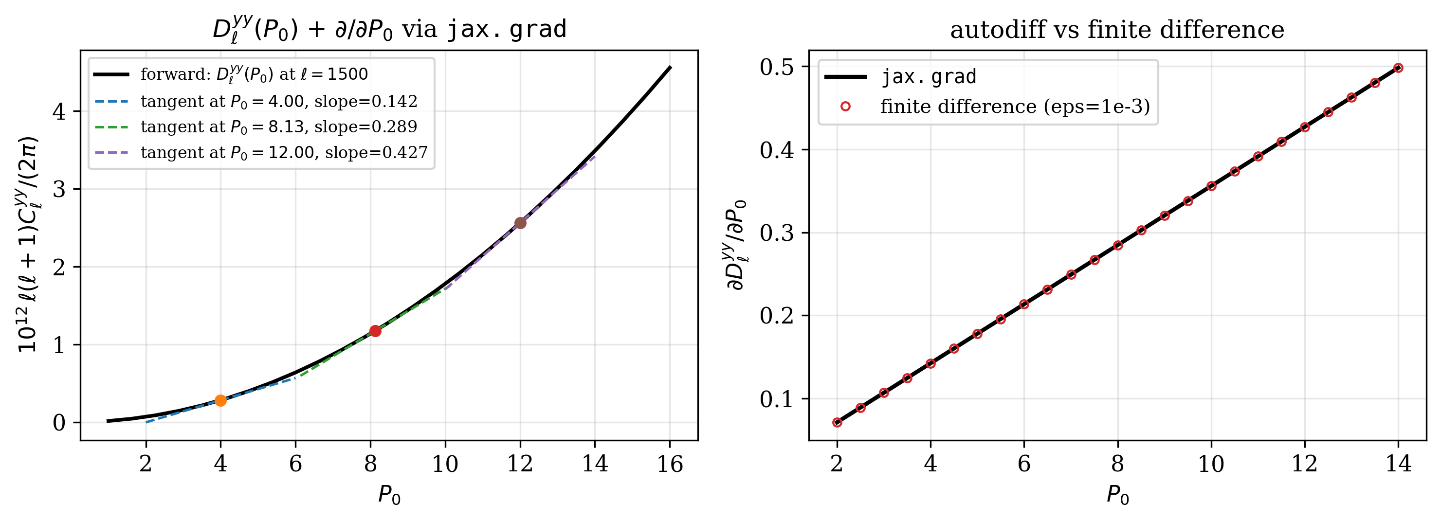
For this benchmark the maximum relative error was \(|\,\mathtt{jax.grad} - \mathtt{FD}\,| / |\,\mathtt{jax.grad}\,| \lesssim 2\times10^{-12}\) — i.e. the gradient is exact to double-precision round-off, which is what you would expect from analytically-derived expressions.

Recommended path: gradient via the factory closure#

For inference at fixed cosmology, the factory closure is by far the fastest way to get \(\partial \boldsymbol{C}^{yy}/\partial \boldsymbol{\theta}_{\rm profile}\):

import jax, jax.numpy as jnp
jax.config.update("jax_enable_x64", True)
import classy_szlite as csl

cosmo = csl.CosmoParams()
ell = jnp.geomspace(2, 5000, 30)
ev = csl.cl_yy_factory(cosmo, ell)        # heavy precomputation, done once

def loss(P0, beta):
    cl_1h, cl_2h = ev(csl.ProfileParamsA10(P0=P0, beta=beta, B=1.25))
    return jnp.sum(cl_1h + cl_2h)

g_P0, g_beta = jax.grad(loss, argnums=(0, 1))(8.13, 5.48)

Warm timing: ~17 ms per gradient call, vs. ~5 ms for the forward pass. The ~3× overhead is the canonical reverse-mode autodiff cost.

Gradient through the full pipeline (cosmology + profile)#

When you also need gradients w.r.t. cosmology, use cl_yy (or any other top-level function) directly:

def full_loss(omega_b, omega_cdm, P0, beta):
    cosmo = csl.CosmoParams(omega_b=omega_b, omega_cdm=omega_cdm)
    profile = csl.ProfileParamsA10(P0=P0, beta=beta, B=1.25)
    cl_1h, cl_2h = csl.cl_yy(cosmo, profile, ell)
    return jnp.sum(cl_1h + cl_2h)

g = jax.grad(full_loss, argnums=(0, 1, 2, 3))(0.0226, 0.118, 8.13, 5.48)

Cold first call ≈ a few seconds (compiles the JAX trace through the cosmology emulator pipeline); warm calls ≈ 50 ms.

Gradient w.r.t. `CosmoParams` as a pytree#

You can differentiate w.r.t. the whole container in one call. JAX returns a CosmoParams whose fields hold the partials:

def cl_loss(cosmo):
    profile = csl.ProfileParamsA10(P0=8.13, beta=5.48, B=1.25)
    cl_1h, cl_2h = csl.cl_yy(cosmo, profile, ell)
    return jnp.sum(cl_1h + cl_2h)

grads = jax.grad(cl_loss)(csl.CosmoParams())
print(grads.omega_b, grads.omega_cdm, grads.fEDE, grads.log10z_c)

Jacobians (Fisher matrix building block)#

Use jax.jacfwd for \(\partial C_\ell/\partial\theta\) when len(ℓ) >> len(θ) (the usual case in cosmology):

def Cl_vec(P0, beta):
    c1, c2 = ev(csl.ProfileParamsA10(P0=P0, beta=beta, B=1.25))
    return c1 + c2

jacobian = jax.jacfwd(Cl_vec, argnums=(0, 1))(8.13, 5.48)
# jacobian[0]: shape (n_ell,)  →  ∂C_ℓ/∂P0
# jacobian[1]: shape (n_ell,)  →  ∂C_ℓ/∂β

For sampled-cosmology Fisher matrices, use the full pipeline:

def Cl_full(omega_b, omega_cdm, P0, beta):
    cosmo = csl.CosmoParams(omega_b=omega_b, omega_cdm=omega_cdm)
    c1, c2 = csl.cl_yy(cosmo, csl.ProfileParamsA10(P0=P0, beta=beta, B=1.25), ell)
    return c1 + c2

J = jax.jacfwd(Cl_full, argnums=(0, 1, 2, 3))(0.0226, 0.118, 8.13, 5.48)
# 4 arrays each of shape (n_ell,) — the columns of the design matrix.

Caveats#

Don’t wrap the factory closure in jax.jit. Internally it calls mcfit.TophatVar for \(\sigma(R)\), which uses NumPy / SciPy code paths that are not jit-safe. The factory is already fast (~5 ms / call) and jax.grad works directly.
For inference at fixed cosmology, prefer the factory path. The full pipeline is gradient-correct but ~3× slower (~50 ms vs ~17 ms with autodiff).
jax.config.update("jax_enable_x64", True) is set on import — cosmology likelihoods need double precision; single precision will give noticeably biased posteriors at the bandpower covariance level.