Tutorials & examples#
Each section pairs a runnable snippet with the figure it produces. All examples assume:
import jax, jax.numpy as jnp
jax.config.update("jax_enable_x64", True)
import numpy as np
import matplotlib.pyplot as plt
import classy_szlite as csl

cosmo = csl.CosmoParams()                      # Planck-18-ish defaults
CMB angular power spectra#
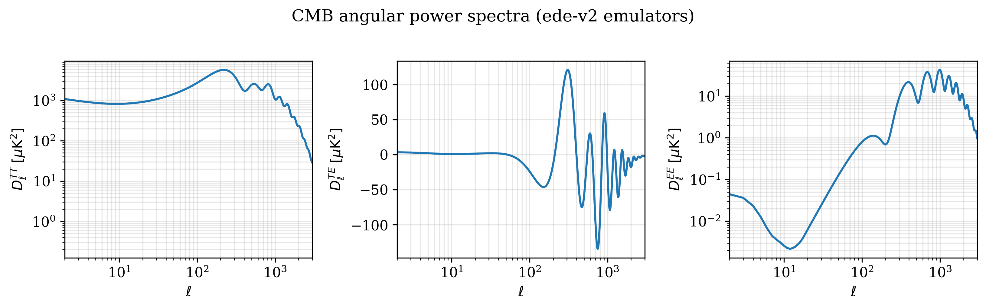
cls = csl.cl_TTTEEE(cosmo, spectra=("tt", "te", "ee"))
T_CMB_uK2 = (2.7255e6) ** 2

fig, axes = plt.subplots(1, 3, figsize=(11, 3.3))
for ax, key, ylab, scale in [
    (axes[0], "tt", r"$D_\ell^{TT}\;[\mu K^2]$", "log"),
    (axes[1], "te", r"$D_\ell^{TE}\;[\mu K^2]$", "linear"),
    (axes[2], "ee", r"$D_\ell^{EE}\;[\mu K^2]$", "log"),
]:
    ax.plot(cls["ell"], cls[key] * T_CMB_uK2)
    ax.set(xscale="log", yscale=scale,
           xlabel=r"$\ell$", ylabel=ylab, xlim=(2, 3000))
    ax.grid(True, alpha=0.3, which="both")
fig.tight_layout()
Matter Pk (linear + nonlinear)#
z_arr = jnp.array([0.0, 0.5, 1.0, 2.0])
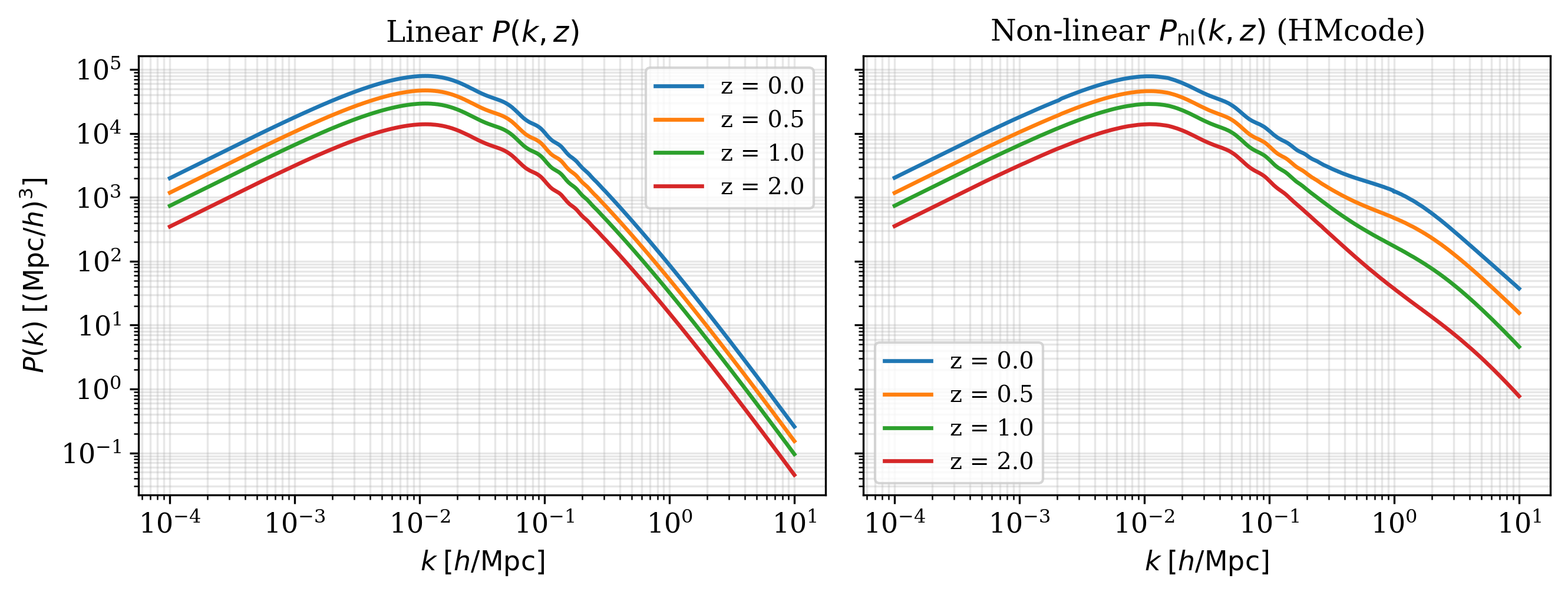
k, pk  = csl.Pk(cosmo,  z_arr)
_, pnl = csl.Pnl(cosmo, z_arr)

fig, axes = plt.subplots(1, 2, figsize=(9, 3.5), sharey=True)
for i, z in enumerate(np.asarray(z_arr)):
    axes[0].loglog(k, pk[i],  label=f"z = {z}")
    axes[1].loglog(k, pnl[i], label=f"z = {z}")
axes[0].set(xlabel=r"$k\;[h/\mathrm{Mpc}]$", ylabel=r"$P(k)\;[(\mathrm{Mpc}/h)^3]$",
            title="Linear")
axes[1].set(xlabel=r"$k\;[h/\mathrm{Mpc}]$", title="Non-linear (HMcode)")
for ax in axes:
    ax.grid(True, which="both", alpha=0.3); ax.legend()
fig.tight_layout()
Cosmological distances#
z = jnp.geomspace(0.01, 5.0, 60)
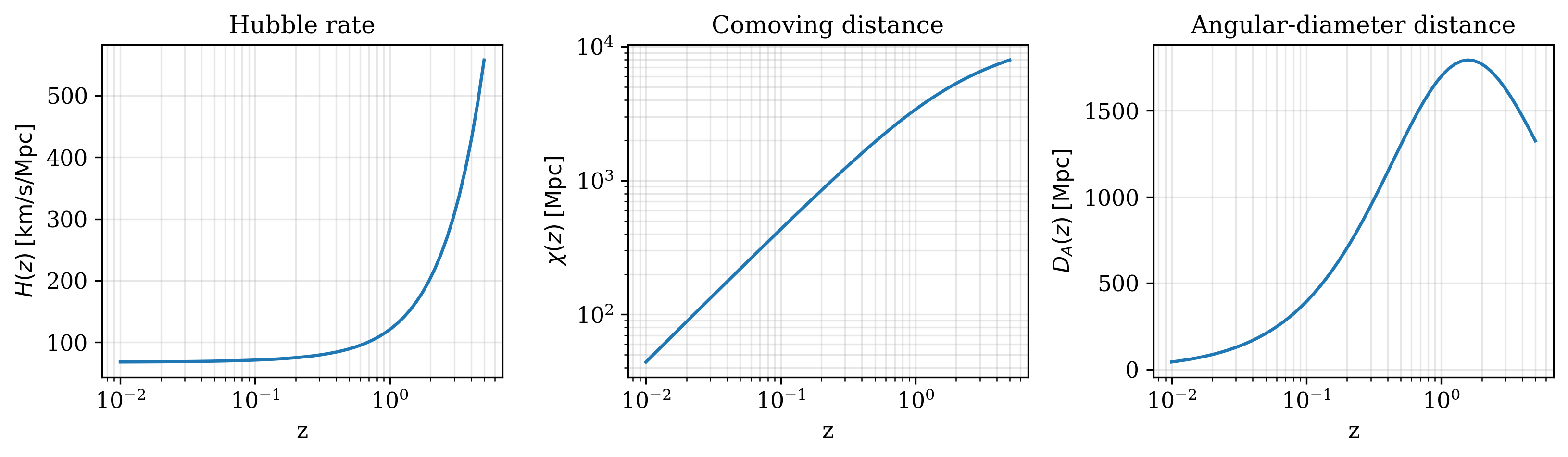
Hz, chi, Da = csl.distances(cosmo, z)
c = 299_792.458

fig, axes = plt.subplots(1, 3, figsize=(11, 3.3))
axes[0].semilogx(z, np.asarray(Hz) * c)
axes[0].set(xlabel="z", ylabel=r"$H(z)\;[\mathrm{km/s/Mpc}]$", title="Hubble rate")
axes[1].loglog(z, chi)
axes[1].set(xlabel="z", ylabel=r"$\chi(z)\;[\mathrm{Mpc}]$", title="Comoving distance")
axes[2].semilogx(z, Da)
axes[2].set(xlabel="z", ylabel=r"$D_A(z)\;[\mathrm{Mpc}]$",
            title="Angular-diameter distance")
for ax in axes: ax.grid(True, alpha=0.3, which="both")
fig.tight_layout()
Linear growth σ₈(z)#
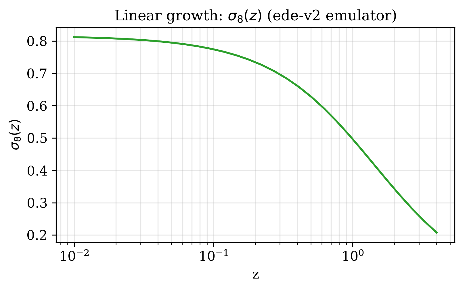
Using the linear \(P_k\) amplitude as a fixed-shape proxy:
z = jnp.geomspace(0.01, 4.0, 30)
k, pk = csl.Pk(cosmo, z)
sigma8_0 = csl.derived(cosmo)["sigma_8"]
amp = np.sqrt(np.trapezoid(pk, k, axis=1))
sigma8_z = sigma8_0 * amp / amp[0]

plt.plot(z, sigma8_z); plt.xscale("log")
plt.xlabel("z"); plt.ylabel(r"$\sigma_8(z)$"); plt.grid(True, alpha=0.3, which="both")
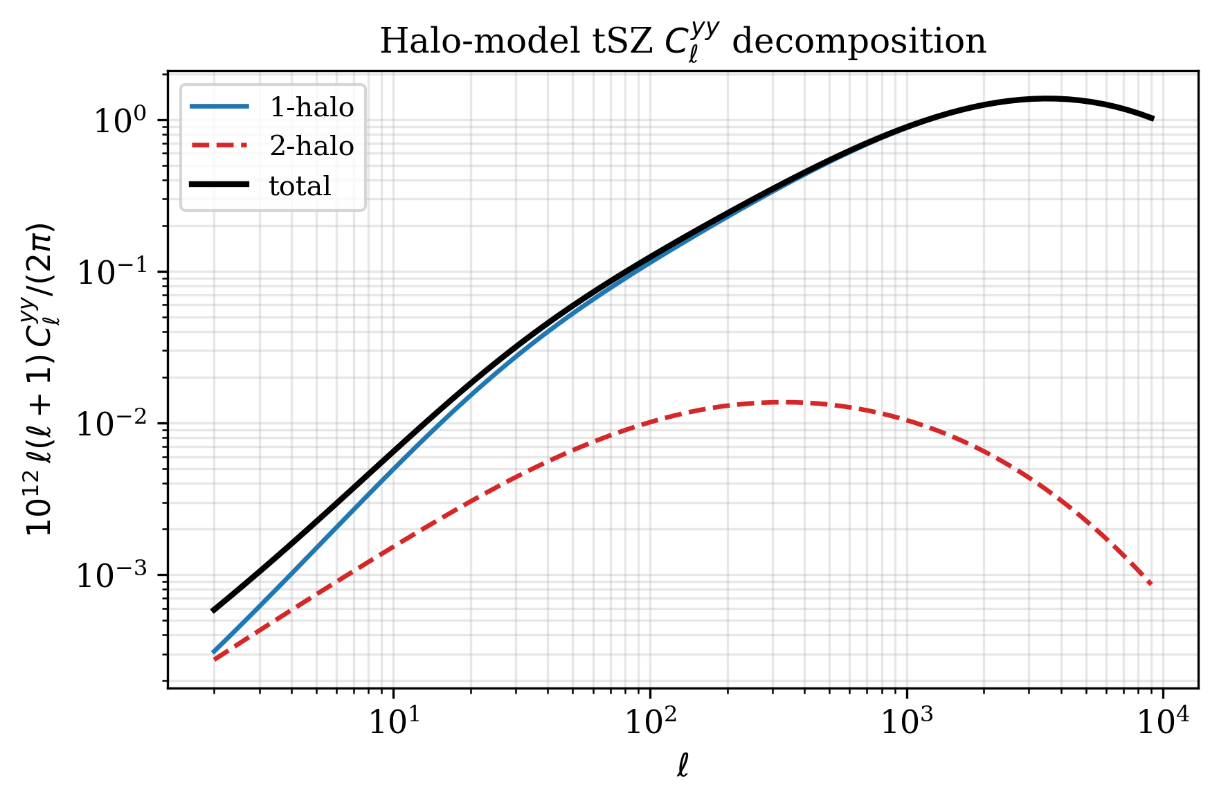
Halo-model tSZ Cl^yy (1h + 2h decomposition)#
profile = csl.ProfileParamsA10(           # Arnaud 2010 universal profile
    P0=8.130, c500=1.156, gamma=0.3292, alpha=1.062, beta=5.4807, B=1.25,
)
ell = jnp.geomspace(2, 9000, 80)
cl_1h, cl_2h = csl.cl_yy(cosmo, profile, ell)

prefac = np.asarray(ell * (ell + 1) / (2 * np.pi)) * 1e12
plt.loglog(ell, prefac * cl_1h,         label="1-halo")
plt.loglog(ell, prefac * cl_2h,         label="2-halo", ls="--")
plt.loglog(ell, prefac * (cl_1h+cl_2h), label="total", color="k", lw=2)
plt.xlabel(r"$\ell$"); plt.ylabel(r"$10^{12}\,\ell(\ell+1)C_\ell^{yy}/(2\pi)$")
plt.grid(True, alpha=0.3, which="both"); plt.legend()
For the dependence on n_z, n_m, m_min, m_max, see the
convergence study.
Battaglia-2012 profile: validation against classy_sz#
classy_szlite’s Battaglia-2012 (B12) GNFW profile is validated against
the reference classy_sz C-code at the same fixed cosmology, matched
physical mass range, and the same Battaglia+2012 fitting coefficients.
ell = jnp.geomspace(100., 5000., 30)
from classy_szlite.api import cosmo_to_dict
from classy_szlite.cosmology import build as build_cg
from classy_szlite.hmf import build_halo_grids
from classy_szlite.power_spectrum import cl_yy_1h_2h

cd = cosmo_to_dict(cosmo)
cg = build_cg(cd, z_grid=jnp.geomspace(0.005, 3.0, 100))
hg = build_halo_grids(cg, cd, delta_crit=200.0,        # M200c HMF for B12
                       m_min=1e10, m_max=3.5e15, n_m=200)

# B12 default fitting coefficients are baked in — pass profile_params=None
@jax.jit
def evaluate():
    return cl_yy_1h_2h(ell, cg, hg, cd, profile='battaglia12',
                       profile_params=None)

cl_1h, cl_2h = evaluate()    # ~4 ms warm on CPU
The full validation script (with classy_sz set-up + timing harness) is
examples/validate_b12.py.
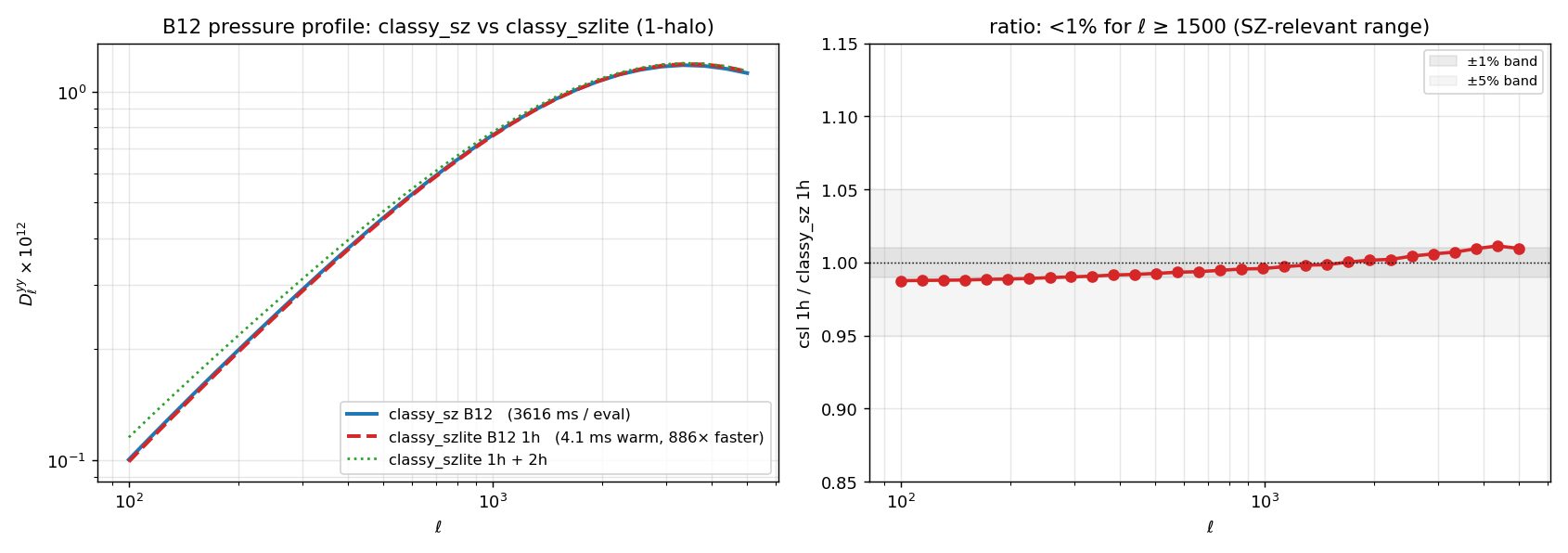
Agreement. Across the full range ℓ ∈ [100, 5000], the two codes match to <1.3% (max), 0.7% mean. The agreement holds from ℓ ≥ 1500 (SZ data range) down to ℓ = 100 (low-ℓ 2-halo regime) — the residual ~1% comes from minor differences in HMF tabulation between the codes.
Important — classy_sz precision settings. Reaching this agreement
requires running classy_sz with n_l_pressure_profile = 500,
n_m_pressure_profile = 500, n_z_pressure_profile = 500,
pressure_profile_epsrel = 1e-4, matching the official
test_classy_sz_clyy_b12_fast.py
test. With the smaller defaults (n_l = 300, ndim_redshifts ~50, etc.) the
classy_sz B12 FFT-tabulation is under-resolved at low ℓ and produces a
spurious ~30% offset at ℓ < 200. This is a numerical convergence
artefact, not a physics difference.
Timing. At fixed cosmology, classy_szlite is ~800× faster per
evaluation than fully-converged classy_sz (~4 ms vs ~3.6 s on CPU),
making it the practical choice for profile-parameter MCMCs at the cost
of a one-off ~2.5 s factory build.
Bandpower covariance: Gaussian + 1-halo trispectrum#
For tSZ, the bandpower covariance has two pieces:
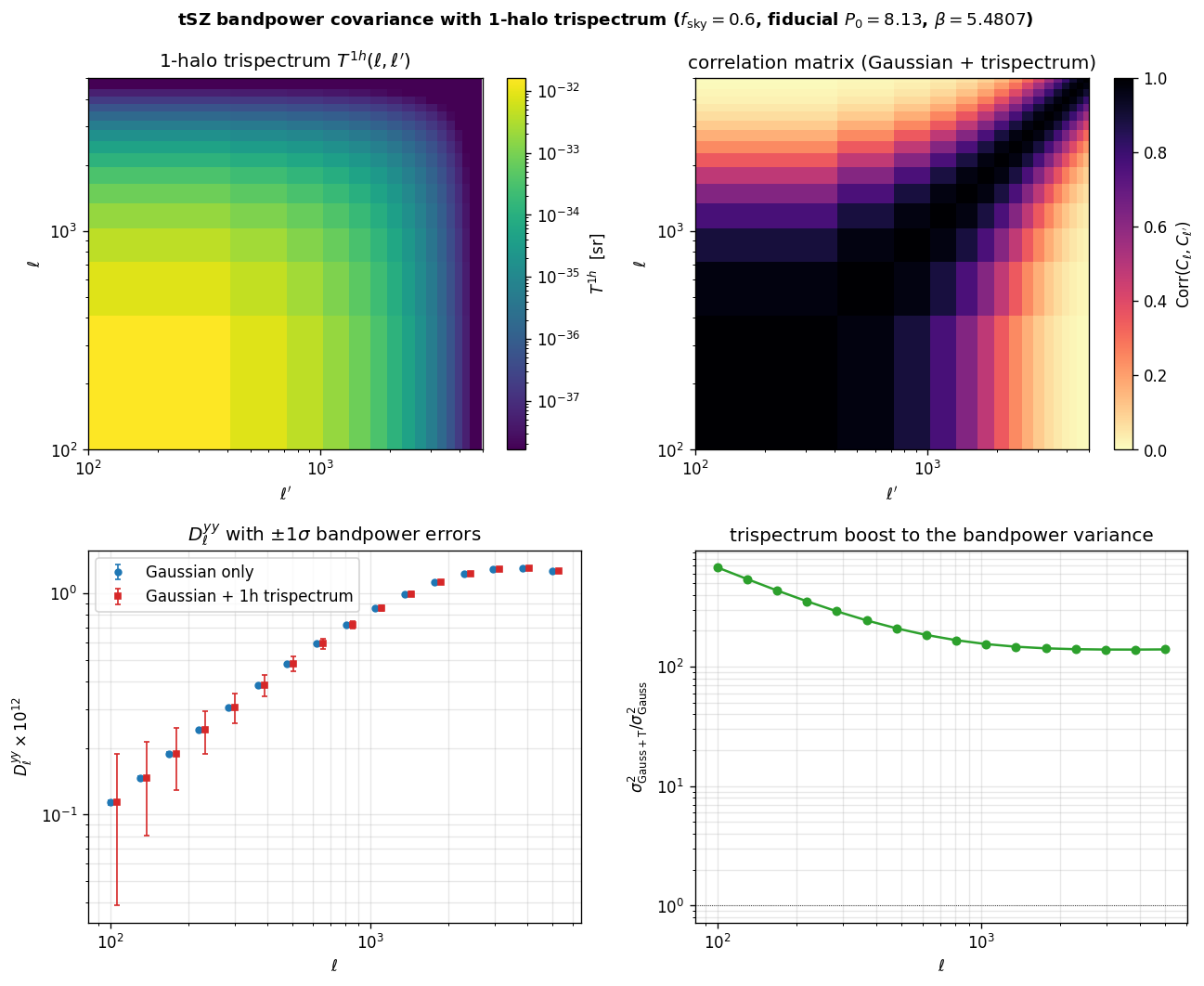
The 1-halo connected trispectrum
is a symmetric (n_ell, n_ell) matrix. For tSZ it dominates the
Gaussian variance by 1–3 orders of magnitude on the diagonal and
introduces strong off-diagonal correlations between bandpower bins
(rare clusters contribute to all multipoles at once).
import jax.numpy as jnp
import classy_szlite as csl

cosmo    = csl.CosmoParams()                                # baseline
fiducial = csl.ProfileParamsA10(                            # A10 universal profile
    P0=8.130, c500=1.156, gamma=0.3292, alpha=1.062, beta=5.4807, B=1.25,
)
ell       = jnp.geomspace(100, 5000, 16)
delta_ell = ell * jnp.log(ell[1] / ell[0])                  # log-bandwidth

# Just the trispectrum (n_ell, n_ell), symmetric:
T = csl.cl_yy_trispectrum(cosmo, fiducial, ell)

# Full bandpower covariance (Gaussian variance + trispectrum):
cov = csl.cl_yy_covariance(cosmo, fiducial, ell, delta_ell,
                            fsky=0.6, include_trispectrum=True)

# Cholesky-ready for synthetic-data generation:
L = jnp.linalg.cholesky(cov)
Diagnostic at the A10 fiducial profile: trispectrum heatmap, full
covariance correlation matrix, σ on D_ℓ × 10¹² with and without the
trispectrum, and the per-bin variance ratio:
Warm timings on a single-core CPU (n_z=100, n_m=200). The cosmology and halo grids are built once and shared between the 1h/2h integrals and the trispectrum contraction:
|
|
|
mem cost ∝ |
|---|---|---|---|
8 |
54 ms |
77 ms |
1.3 M floats |
16 |
64 ms |
93 ms |
5.1 M floats |
32 |
90 ms |
139 ms |
21 M floats |
cl_yy_covariance takes ~25–50 ms more than cl_yy_trispectrum
alone because it also runs the 1h+2h cl_yy integral (the 2-halo
term needs an extra P_lin(k_ℓ, z) interpolation that the
trispectrum doesn’t). Both functions reuse the same emulator forward
pass and halo-grid build. Typical bandpower counts (8–30) cost
<0.2 s including the full covariance assembly.
Note on units. cl_yy_covariance returns the covariance on the
dimensionless C_ℓ. If your data vector is in D_ℓ × 10¹² (the
standard plotting convention), rescale by the outer product of the
prefactor before Cholesky:
dl_factor = ell * (ell + 1) / (2 * jnp.pi) * 1e12
cov_Dell  = cov * (dl_factor[:, None] * dl_factor[None, :])
L         = jnp.linalg.cholesky(cov_Dell)
Bestfit + NUTS + RW-MH on synthetic Cl^yy bandpowers (baseline cosmology)#
The factory closure makes both gradient-based optimisation (L-BFGS)
and Hamiltonian-style samplers (NUTS) a natural fit: each forward
pass is one ~5 ms ev(profile) call, gradients are exact via
jax.grad, and there is no proposal-covariance tuning.
We build a fully self-contained inference example at a fixed baseline cosmology (Planck-18-like, σ₈ ≈ 0.81) by:
Generating synthetic bandpowers at a fiducial Arnaud-10 profile via a Cholesky decomposition of the analytic tSZ bandpower covariance (Gaussian variance + 1-halo connected trispectrum) — one call to
classy_szlite.cl_yy_covariance. For tSZ the trispectrum dominates the Gaussian variance by ~300–1000× on the diagonal, so leaving it out would massively under-state the error bars.L-BFGS bestfit of (P₀, β) via
scipy.optimize.minimizewith exactjax.gradgradients — converges in ~30–40 fn evals, < 0.5 s.NumPyro NUTS for the full posterior, initialised at the bestfit — reaches a publication-grade posterior (|Z| < 0.1σ vs gold-standard, R-hat < 1.05) in ~10 s wall.
cobaya RW-MH for sampler-vs-sampler comparison — typically ~10–15 min wall single-core to converge to R-1 = 0.01.
import jax, jax.numpy as jnp
jax.config.update("jax_enable_x64", True)
import numpy as np, scipy.optimize as so
import numpyro, numpyro.distributions as dist
from numpyro.infer import MCMC, NUTS
import classy_szlite as csl

# --- baseline cosmology + fiducial profile ---
cosmo    = csl.CosmoParams(omega_b=0.0226, omega_cdm=0.118,
                           H0=68.22, tau_reio=0.0561,
                           ln10_10_As=3.060, n_s=0.9743)
fiducial = csl.ProfileParamsA10(           # Arnaud 2010 universal profile
    P0=8.130, c500=1.156, gamma=0.3292, alpha=1.062, beta=5.4807, B=1.25,
)

# --- log-spaced ell-binning ---
ell       = jnp.geomspace(100.0, 5000.0, 8)
delta_ell = ell * jnp.log(ell[1] / ell[0])         # bandwidth per bin
fsky      = 0.6

# --- analytic covariance (Gaussian + 1h trispectrum) ---
# cl_yy_covariance returns the covariance on the DIMENSIONLESS C_ell;
# the data we'll generate is in D_ell × 1e12 units, so we rescale by
# (dl_factor ⊗ dl_factor) before Cholesky.
ev          = csl.cl_yy_factory(cosmo, ell)        # JIT'd fast closure
dl_factor   = ell * (ell + 1) / (2 * jnp.pi) * 1e12
cov_cl      = csl.cl_yy_covariance(cosmo, fiducial, ell, delta_ell, fsky=fsky)
cov_dell    = cov_cl * (dl_factor[:, None] * dl_factor[None, :])    # → D_ell × 1e12 units

# Inflate the covariance to widen the posterior and make the
# (P_0, β) degeneracy direction visible in the corner plot. With
# noise_factor = 1 the constraint is so tight that the posterior
# collapses to a near-point estimate at the fiducial; 9 (i.e. 3×
# the per-bin σ) gives ~5% relative widths on P_0 and β.
noise_factor = 9
cov     = cov_dell * noise_factor
inv_cov = jnp.linalg.inv(cov)
L_chol  = jnp.linalg.cholesky(cov)

# Trispectrum vs Gaussian-only on the diagonal (sanity print)
cov_g_cl = csl.cl_yy_covariance(cosmo, fiducial, ell, delta_ell,
                                 fsky=fsky, include_trispectrum=False)
print("trispectrum / Gaussian variance per bin:",
      np.round(np.diag(np.asarray(cov_cl)) / np.diag(np.asarray(cov_g_cl)), 1))

# --- generate one synthetic D_ell^yy realisation ---
c1, c2    = ev(fiducial)
Dell_fid  = dl_factor * (c1 + c2)
key       = jax.random.PRNGKey(42)
Dell_data = Dell_fid + L_chol @ jax.random.normal(key, ell.shape)
# To use real ACT / Planck data instead: replace the three lines
# above with a loader that returns (ell, Dell_data, cov) from disk
# (and drop the `noise_factor` inflation — real data carries its
# real uncertainty already).

def forward(P0, beta):
    prof = csl.ProfileParamsA10(P0=P0, c500=1.156, gamma=0.3292,
                                 alpha=1.062, beta=beta, B=1.25)
    c1, c2 = ev(prof)
    return dl_factor * (c1 + c2)

# 1) L-BFGS bestfit with JAX gradients
def neg_log_like(x):
    r = Dell_data - forward(x[0], x[1])
    return 0.5 * r @ inv_cov @ r
nll, gnll = jax.jit(neg_log_like), jax.jit(jax.grad(neg_log_like))
bf = so.minimize(lambda x: float(nll(x)), [8.13, 5.48],
                 jac=lambda x: np.asarray(gnll(x)),
                 method="L-BFGS-B", bounds=[(0.1, 20), (0.5, 10)])
print(f"bestfit:   P0={bf.x[0]:.2f}  β={bf.x[1]:.2f}  χ²={2*bf.fun:.1f}/6")

# 2) NUTS, init at bestfit
def model():
    P0   = numpyro.sample("P0",   dist.Uniform(0.0, 20.0))
    beta = numpyro.sample("beta", dist.Uniform(0.0, 10.0))
    r    = Dell_data - forward(P0, beta)
    numpyro.factor("loglike", -0.5 * r @ inv_cov @ r)

mcmc = MCMC(NUTS(model, dense_mass=True),
            num_warmup=100, num_samples=200, num_chains=2,
            chain_method="sequential", progress_bar=False)
mcmc.run(jax.random.PRNGKey(0),
         init_params={"P0":   jnp.full(2, float(bf.x[0])),
                      "beta": jnp.full(2, float(bf.x[1]))})
s = mcmc.get_samples()
print(f"NUTS:      P0={s['P0'].mean():.2f}±{s['P0'].std():.2f}  "
      f"β={s['beta'].mean():.2f}±{s['beta'].std():.2f}")
Typical output on a single-core CPU (warm closure, JIT compiled) —
the synthetic posterior is centred on the A10 fiducial by construction;
with noise_factor = 9 the σ on each parameter is large enough to
expose the (P_0, β) degeneracy direction:
trispectrum / Gaussian variance per bin: [1455. 904. 591. 423. 340. 307. 298. 298.]
bestfit:     P0=8.01 (fid 8.13)  β=5.42 (fid 5.48)  χ²=5.2/6    (16 fn evals, ~0.4 s)
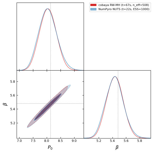
NUTS:        P0=8.04±0.33        β=5.43±0.13        corr=+0.99
             ESS≈900, R-hat=1.001                              (~22 s wall, 2 chains × 1300 samples)
cobaya RW-MH: P0=8.04±0.30        β=5.44±0.12        n_eff(Kish)≈508
              R-1=0.05 stopping criterion                       (~67 s wall, single chain)
The synthetic-data path is fully reproducible — you only need
classy_szlite + numpyro + scipy, no external bandpower files.
Swap in real bandpowers by replacing the three lines that build
ell, Dell_data, and cov; everything downstream is unchanged.
Triangle plot of the recovered posterior. cobaya RW-MH (red) and NumPyro NUTS (blue) on the same synthetic-data likelihood agree to within sampling noise — same mean, same width, same +0.99 (P_0, β) degeneracy direction. The dashed gridlines mark the A10 fiducial truth; both posteriors contain it within the 1σ contour. At equal-quality convergence, NUTS reaches publication-grade ~3× faster wall-for-wall on this 2D problem (see paper Fig. 7 for the systematic comparison across budgets):
The full runnable script (synthetic data + bestfit + NUTS + MH overlay
plotting) is at
examples/nuts_clyy_profile.py.
Posterior bands on the GNFW pressure profile#
Since (P₀, β) are the only GNFW parameters sampled in the fit above, each posterior sample maps to a different dimensionless profile
Drawing random samples from the NUTS posterior and taking the 16/50/84 percentiles gives a median curve + 1σ band. Plotted together with the fiducial A10 profile and a \(\,p(x)\,x^2\) y-axis (which flattens the inner power-law fall-off and makes the outer slope β easy to read):
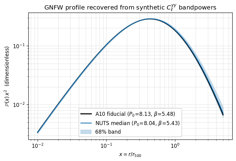
With synthetic data generated at the A10 fiducial profile (this docs
example uses noise_factor = 9 to inflate the bandpower covariance —
see the inference example above), the NUTS-recovered median sits on
top of the A10 fiducial by construction; the 1σ band shows the
posterior uncertainty propagated through the GNFW shape.
The runnable script is at
examples/profile_bands.py.
Fisher matrix in one autodiff sweep#
For a Gaussian likelihood with fixed covariance \(\Sigma\), the Fisher matrix at parameter point \(\boldsymbol{\theta}\) is
with \(\mu(\boldsymbol{\theta}) = \) forward\((P_0, \beta)\). The Jacobian
\(J = \partial \mu / \partial \boldsymbol{\theta}\) is exactly what
jax.jacfwd returns in a single forward-mode autodiff sweep — no
finite-difference loop, no \(\varepsilon\) tuning.
import jax, jax.numpy as jnp
import classy_szlite as csl

forward = build_forward(cosmo, ell)   # see nuts_clyy_profile.py

def mu(x):
    return forward(x[0], x[1])

J = jax.jit(jax.jacfwd(mu))(jnp.asarray([P0_bf, beta_bf]))    # (n_bp, 2)
F = J.T @ inv_cov @ J                                          # (2, 2)
cov_fisher = jnp.linalg.inv(F)
The examples/fisher_clyy_profile.py script runs this end-to-end and
overlays the 68%/95% Fisher ellipses on the NUTS posterior:
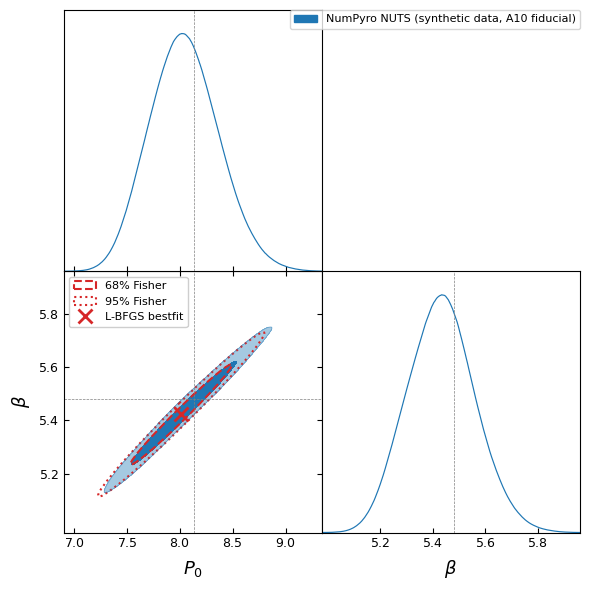
Wall time: ~135 ms per Fisher matrix after JAX warmup (10-run average, including jit dispatch). The autodiff Fisher matches a 2-point central finite-difference reference (\(\varepsilon = 10^{-3}\)) to \(|\Delta F|/|F| \sim 10^{-6}\). With synthetic A10-fiducial data the posterior is nearly Gaussian, so the Fisher 68%/95% ellipses match the NUTS contours to within ~3 % on the marginal widths (σ_Fisher = 0.316 vs σ_NUTS = 0.326 for \(P_0\); σ_Fisher = 0.124 vs σ_NUTS = 0.128 for \(\beta\)). When the posterior is non-Gaussian (skewed tails, multi-modality), the Fisher approximation will under-estimate the uncertainty — a useful sanity check for forecasting.
The runnable script is at
examples/fisher_clyy_profile.py.
End-to-end MCMC pattern (cobaya Theory)#
For the RW-MH cobaya baseline that the NUTS example above reproduces,
the natural cobaya Theory shape is:
from cobaya.theory import Theory
import classy_szlite as csl
import numpy as np, jax, jax.numpy as jnp
jax.config.update("jax_enable_x64", True)

class MyTSZTheory(Theory):
    # The standard 6 cosmology parameters — fixed for this Theory
    omega_b:    float = 0.0226
    omega_cdm:  float = 0.118
    H0:         float = 68.22
    tau_reio:   float = 0.0561
    ln10_10_As: float = 3.06
    n_s:        float = 0.9743

    multipoles_file: str = None       # required: 1 ell per line

    params = {"P0GNFW": 8.13, "c500": 1.156, "gammaGNFW": 0.3292,
              "alphaGNFW": 1.062, "betaGNFW": 5.48, "B": 1.25}

    def initialize(self):
        ell = jnp.asarray(np.loadtxt(self.multipoles_file))
        cosmo = csl.CosmoParams(
            omega_b=self.omega_b, omega_cdm=self.omega_cdm,
            H0=self.H0, tau_reio=self.tau_reio,
            ln10_10_As=self.ln10_10_As, n_s=self.n_s,
        )
        self._csl = csl
        self._eval = csl.cl_yy_factory(cosmo, ell)   # heavy work, done once
        self._ell_np = np.asarray(ell)
        self._dl_factor = ell * (ell + 1) / (2 * jnp.pi) * 1e12

    def get_can_provide(self): return ["Cl_sz"]

    def calculate(self, state, want_derived=True, **p):
        prof = self._csl.ProfileParamsA10(
            P0=p["P0GNFW"], c500=p["c500"],
            gamma=p["gammaGNFW"], alpha=p["alphaGNFW"],
            beta=p["betaGNFW"], B=p["B"],
        )
        cl1, cl2 = self._eval(prof)
        state["Cl_sz"] = {
            "ell": self._ell_np,
            "1h":  np.asarray(self._dl_factor * cl1),
            "2h":  np.asarray(self._dl_factor * cl2),
        }

    def get_Cl_sz(self):
        return self._current_state["Cl_sz"]
A complete worked example with this MyTSZTheory paired with a Gaussian
likelihood (ACT-DR6 may26 setup) converges in ~2 min wall for
~10,000 samples (R−1 = 0.008, 4-way MPI, Rminus1_stop = 0.01).
Cosmology scan#
import classy_szlite as csl
import numpy as np

omega_cdm_vals = np.linspace(0.10, 0.14, 5)
for omega_cdm in omega_cdm_vals:
    cosmo = csl.CosmoParams(omega_cdm=float(omega_cdm))
    d = csl.derived(cosmo)
    print(f"omega_cdm = {omega_cdm:.3f}  →  σ8 = {d['sigma_8']:.4f}, "
          f"Ω_m = {d['Omega_m']:.4f}")
Exploring EDE space#
The v2 emulator suite spans early-dark-energy parameter space; set
fEDE, log10z_c, thetai_scf to non-default values to leave the
LCDM-equivalent point:
ede_cosmo = csl.CosmoParams(
    fEDE=0.10, log10z_c=3.5, thetai_scf=2.83,
)
csl.derived(ede_cosmo)
# → σ8 drops as fEDE rises (more EDE → less time for growth)
Pre-compiling a forward + gradient function#
For a parameter-inference pipeline that calls both the forward and the gradient many times, JAX naturally caches the compiled trace:
import jax, jax.numpy as jnp
import classy_szlite as csl

cosmo = csl.CosmoParams()
ell = jnp.geomspace(2, 9000, 80)
ev = csl.cl_yy_factory(cosmo, ell)

def D_ell(P0, beta):
    profile = csl.ProfileParamsA10(P0=P0, beta=beta, B=1.25)
    cl1, cl2 = ev(profile)
    return ell * (ell + 1) / (2 * jnp.pi) * (cl1 + cl2) * 1e12

dl     = D_ell(8.13, 5.48)                                                       # ~5 ms
g_P0   = jax.grad(lambda P0, b: jnp.sum(D_ell(P0, b)), argnums=0)(8.13, 5.48)    # ~17 ms warm
g_beta = jax.grad(lambda P0, b: jnp.sum(D_ell(P0, b)), argnums=1)(8.13, 5.48)
EDE NUTS demo — recovering an MCMC posterior in 3 hours#
This walks through the most ambitious validation we have run with
classy_szlite so far: reproducing the ACT-DR6 + Planck early dark energy
(EDE) posterior with HMC (No-U-Turn Sampler), and comparing the result
against the published RW-MH chain that originally fit the data.
The full reference for everything below — chain configuration, scripts, log
files, posterior triangles, timing breakdowns — is the report at
docs/_static/ede_nuts_report.md.
Pipeline at a glance#
Theory. Cosmological observables come from
classy_szlite’s ede-v2 CosmoPower emulator (CMB TT/TE/EE through ℓ_max = 9 500, used via the new :func:~classy_szlite.cl_TTTEEE_jaxfunction with theclassy_szfastℓ-convention).Likelihoods. The same four cobaya likelihoods used by the reference chain, but re-implemented in JAX inside the new :mod:
classy_szlite.likelihoodssub-package — see :func:~classy_szlite.likelihoods.chi2_lowTT, :func:~classy_szlite.likelihoods.chi2_sroll2, :func:~classy_szlite.likelihoods.chi2_placand :func:~classy_szlite.likelihoods.chi2_mflike_v2.Foreground marginalisation. The 11 amplitudes that enter linearly (
a_kSZ, a_p, a_s, a_tSZ, a_c, a_gtt, a_gee, a_psee, a_pste, a_gte, xi) are sampled; SED tilts and bandpass shifts are held at the chain best-fit. See :func:~classy_szlite.likelihoods.fg_totals_jax.Sampler. NumPyro NUTS, 4 parallel chains,
dense_mass=True,target_accept_prob=0.9,max_tree_depth=11, 800 warmup + 3 000 samples per chain.
Setting up the data tables#
The JAX likelihoods need a small number of pre-computed tables (bandpowers,
covariances, window functions, fixed foreground at best-fit). Extract them
once on a machine where cobaya plus the relevant data packages are
installed:
python -m classy_szlite.likelihoods.extract_data \
    --chain-yaml /path/to/p-actbase_ede+n3_classsz.input.yaml \
    --packages-path ~/cobaya_packages
That writes ~/.classy_szlite/likelihood_data.npz (~150 MB) and
~/.classy_szlite/mflike_fg_components.npz (~25 MB). Subsequent calls
load them automatically; alternatively set
CLASSY_SZLITE_LIKELIHOOD_DATA to point elsewhere.
Running NUTS#
import jax, jax.numpy as jnp
import numpyro
import numpyro.distributions as dist
from numpyro.infer import NUTS, MCMC

import classy_szlite as csl
from classy_szlite.likelihoods import total_chi2

UNIFORM_BOUNDS = {
    "omega_b": (0.017, 0.027), "omega_cdm": (0.09, 0.15), "H0": (40.0, 99.0),
    "fEDE": (0.001, 0.5), "log10z_c": (3.0, 4.3), "thetai_scf": (0.1, 3.1),
    "logA": (2.5, 3.5), "n_s": (0.9, 1.1), "tau_reio": (0.0, 0.1),
    # ... + 29 nuisance bounds; see scripts/jax_priors.py in the test repo.
}

def neg2_loglike(p):
    cosmo = {
        "H0": p["H0"], "omega_b": p["omega_b"], "omega_cdm": p["omega_cdm"],
        "ln10_10_As": p["logA"], "n_s": p["n_s"], "tau_reio": p["tau_reio"],
        "fEDE": p["fEDE"], "log10z_c": p["log10z_c"], "thetai_scf": p["thetai_scf"],
        "m_ncdm": 0.02, "N_ur": 0.00441,
    }
    return total_chi2(cosmo, p, use_v2_foregrounds=True)

def model():
    p = {n: numpyro.sample(n, dist.Uniform(lo, hi))
         for n, (lo, hi) in UNIFORM_BOUNDS.items()}
    numpyro.factor("loglike", -0.5 * neg2_loglike(p))

kernel = NUTS(model, target_accept_prob=0.9, max_tree_depth=11, dense_mass=True)
mcmc = MCMC(kernel, num_warmup=800, num_samples=3000, num_chains=4,
            chain_method="parallel", progress_bar=True)
mcmc.run(jax.random.PRNGKey(0))
samples = mcmc.get_samples(group_by_chain=True)
On a Mac M4 (10 performance cores, 4 chains running in parallel) this completes in ≈ 3 hours. All chains satisfy R-hat ≤ 1.012 with a median divergence rate of 1.7 %.
Result#
Recovered cosmology marginals match the reference MH-RW chain to well within 1 σ on every parameter — including the non-Gaussian, near- prior-boundary
fEDEdistribution.τ-shift in early NUTS runs (v2 NUTS gave τ = 0.0649 vs reference 0.0599) vanishes once the
classy_szfastℓ-convention is used in :func:classy_szlite.cl_TTTEEE_jax(now the default).Wall-clock: ~3 h for
classy_szliteNUTS, ~18 days for the RW-MH reference chain on the same hardware class — a ~140× speedup at the same statistical precision.
The full report has the corner plots, R-hat / ESS tables, per-component
timing breakdowns and a discussion of where the speed-up came from (the
mflike.BandpowerForeground Python overhead, mostly).
The tSZ “y-kernel”: where the Compton-y power spectrum comes from#
A classic class_sz diagnostic (class_sz_szkernel.ipynb) is the tSZ kernel — the integrand of the 1-halo Compton-y power spectrum in the (redshift, halo-mass) plane at a fixed multipole. The 1-halo term is
C_\ell^{yy,\,1h} = \int dz\, \frac{dV}{dz\,d\Omega}
    \int d\ln M\, \frac{dn}{d\ln M}\, |y_\ell(M,z)|^2 ,
so the quantity under the double integral,
\frac{d^2 C_\ell^{yy}}{dz\, d\ln M}
    = \frac{dV}{dz\,d\Omega}\,\frac{dn}{d\ln M}\,|y_\ell(M,z)|^2 ,
tells you which haloes source the signal at a given scale.
classy_szlite exposes exactly these pieces — _y_ell_grid returns
y_ell(ℓ, z, M) and the volume element dV/dzdΩ, while the halo grids carry
dn/dlnM. The kernel is then a one-line product:
import jax.numpy as jnp
import classy_szlite as csl
from classy_szlite.api import cosmo_to_dict
from classy_szlite.cosmology import build as build_cosmo_grids
from classy_szlite.hmf import build_halo_grids
from classy_szlite.power_spectrum import _y_ell_grid

cosmo = csl.CosmoParams(omega_b=0.02242, omega_cdm=0.11933, H0=67.66,
                        ln10_10_As=3.047, n_s=0.9665, tau_reio=0.0561)
cd = cosmo_to_dict(cosmo)
cg = build_cosmo_grids(cd, z_grid=jnp.linspace(0.01, 5.0, 300))
hg = build_halo_grids(cg, cd, delta_crit=200.0, m_min=1e10, m_max=1e15, n_m=300)

y_ell, dVdz = _y_ell_grid(jnp.asarray([10000.0]), cg, hg, cd,
                          profile="battaglia12", profile_params=None)
kernel = dVdz[None, :, None] * hg.dndlnm[None, :, :] * y_ell ** 2   # (ℓ, z, M)
Plotting kernel with cmap='hot' (x = log₁₀M, y = z) reproduces the
class_sz SZ-kernel heat-map:
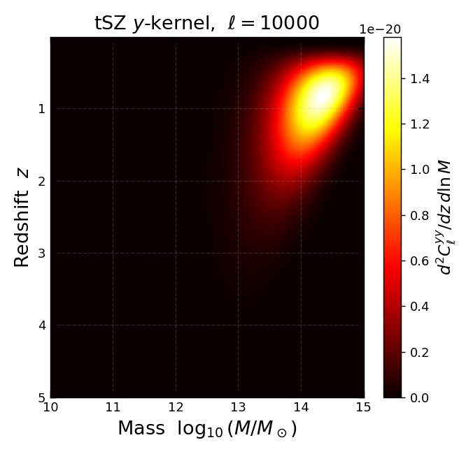
As the multipole increases, the bright region migrates from massive, nearby clusters (large angular scales) toward lower-mass, higher-redshift haloes (small angular scales):
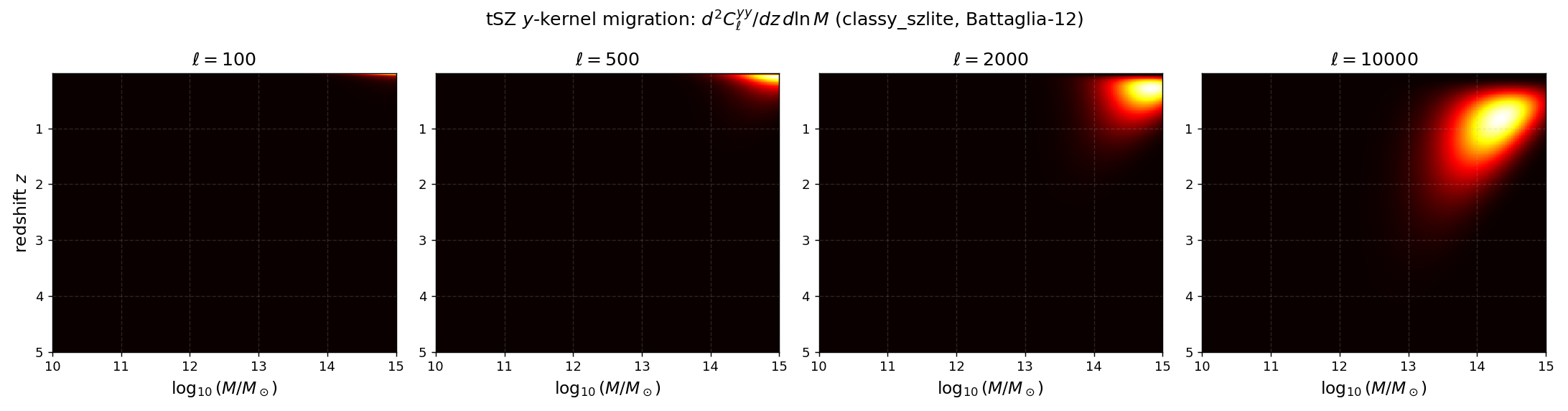
Full script: examples/sz_kernel.py.