Cl^yy convergence#
cl_yy and cl_yy_factory integrate the halo model over redshift and
halo mass. Two discretisation grids (n_z, n_m) and two cut-offs
(m_min, m_max) drive the residual numerical error. The defaults are
chosen so that the total error is well below \(10^{-3}\) — adequate for any
foreseeable bandpower covariance — but you may want tighter or looser
settings for forecasts vs. real data.
What was measured#
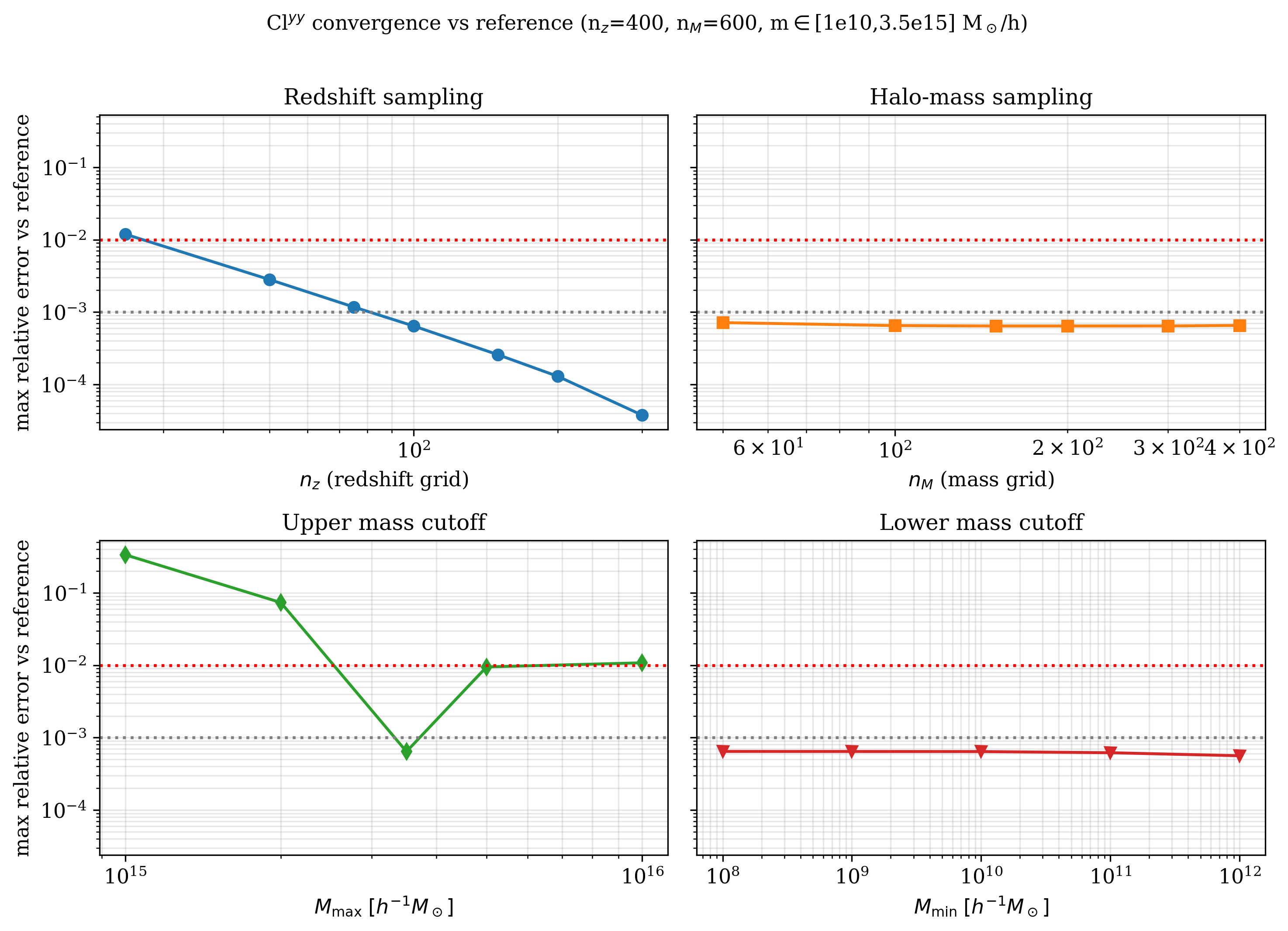
We compute \(\bigl(\Delta C_\ell^{yy}/C_\ell^{yy}\bigr)_{\max}\) across \(\ell \in [100, 8000]\) (12 log-spaced bins), using
profile: Arnaud-10 with \((P_0=8.13,\,\beta=5.48,\,B=1.25)\)
cosmology: ede-v2 LCDM-equivalent (defaults)
against a high-resolution reference of \(n_z = 400,\,n_M = 600,\, M \in [10^{10},\,3.5\times10^{15}]\,M_\odot/h\).
Numerical results#
|
max \(\lvert\Delta C/C\rvert\) |
|---|---|
25 |
1.2 × 10⁻² |
50 |
2.8 × 10⁻³ |
75 |
1.2 × 10⁻³ |
100 (default) |
6.4 × 10⁻⁴ |
150 |
2.6 × 10⁻⁴ |
200 |
1.3 × 10⁻⁴ |
300 |
3.8 × 10⁻⁵ |
|
max \(\lvert\Delta C/C\rvert\) |
|---|---|
50 |
7.2 × 10⁻⁴ |
100 |
6.5 × 10⁻⁴ |
150 |
6.4 × 10⁻⁴ |
200 (default) |
6.4 × 10⁻⁴ |
300 |
6.4 × 10⁻⁴ |
400 |
6.5 × 10⁻⁴ |
n_m is saturated by ~100: the integrand decays steeply away from the
characteristic mass scale, so doubling the grid past that has no effect.
\(M_{\rm max}\) (\(M_\odot/h\)) |
max \(\lvert\Delta C/C\rvert\) |
|---|---|
1 × 10¹⁵ |
3.4 × 10⁻¹ (truncation, miss massive halos) |
2 × 10¹⁵ |
7.4 × 10⁻² (truncation) |
3.5 × 10¹⁵ (default) |
6.4 × 10⁻⁴ |
5 × 10¹⁵ |
9.5 × 10⁻³ (slight extra discretisation error) |
1 × 10¹⁶ |
1.1 × 10⁻² (slight extra discretisation error) |
\(M_{\rm min}\) (\(M_\odot/h\)) |
max \(\lvert\Delta C/C\rvert\) |
|---|---|
1 × 10⁸ |
6.4 × 10⁻⁴ |
1 × 10⁹ |
6.4 × 10⁻⁴ |
1 × 10¹⁰ (default) |
6.4 × 10⁻⁴ |
1 × 10¹¹ |
6.2 × 10⁻⁴ (small structure in low-z 2-halo) |
1 × 10¹² |
5.6 × 10⁻⁴ |
m_min matters very little (low-mass halos contribute negligibly to tSZ).
Recommended settings#
Use case |
|
|
|
|
target accuracy |
|---|---|---|---|---|---|
MCMC / production (default) |
100 |
200 |
1 × 10¹⁰ |
3.5 × 10¹⁵ |
≤ 10⁻³ |
Fast forecast / pre-MCMC |
50 |
100 |
1 × 10¹⁰ |
3.5 × 10¹⁵ |
≤ 3 × 10⁻³ |
Reference / cross-check |
300 |
200 |
1 × 10¹⁰ |
3.5 × 10¹⁵ |
≤ 10⁻⁴ |
Quick smoke-test |
25 |
50 |
1 × 10¹⁰ |
3.5 × 10¹⁵ |
~ 1 × 10⁻² |
Caveats and notes#
Don’t lower \(M_{\rm max}\) below \(3 \times 10^{15}\): the massive end of the HMF still contributes a few percent to the 1-halo term.
The seeming rise of the error for \(M_{\rm max} \gtrsim 5\times10^{15}\) is a discretisation artefact: the same \(n_m\) has to span a much larger \(\log M\) range, so the per-bin resolution drops. If you want a wider mass range, raise
n_mproportionally.\(\sigma(R)\) is computed via
mcfit.TophatVar, which requires a uniformly log-spaced \(k\) grid. The grid is hardcoded to match the ede-v2 emulator’s \(k\) range (down to \(k=10^{-4}\) after low-\(k\) \(k^{n_s}\) extrapolation), so there is nok_min/k_maxknob to tune. The convergence above already accounts for this fixed grid.
How to reproduce#
import numpy as np, jax.numpy as jnp
import classy_szlite as csl

cosmo = csl.CosmoParams()
profile = csl.ProfileParamsA10(P0=8.13, beta=5.48, B=1.25)
ell = jnp.geomspace(100, 8000, 12)

def total(**kw):
    c1, c2 = csl.cl_yy(cosmo, profile, ell, **kw)
    return np.asarray(c1 + c2)

ref = total(n_z=400, n_m=600)

for nz in [25, 50, 75, 100, 150, 200, 300]:
    cur = total(n_z=nz, n_m=200)
    err = np.max(np.abs(cur - ref) / np.abs(ref))
    print(f"n_z={nz:4d}  max |ΔC/C| = {err:.2e}")